import pandas as pd
import sqlite3

# Use 'with' to ensure the connection is properly closed after use
with sqlite3.connect("resources/mlb2023.db") as conn:
    # Write your SQL query
    query = "SELECT * FROM batting"

    # Read data from the database into a pandas DataFrame
    mlb = pd.read_sql_query(query, conn)


with sqlite3.connect("resources/mlbpost2023.db") as conn:
    # Write your SQL query
    query = "SELECT * FROM batting"

    # Read data from the database into a pandas DataFrame
mlbpost = pd.read_sql_query(query, conn)6 Creating Visualisation with Python
7 Analyse Shehei Ohtani’s Performance
In this chapter, we want to explore some common charts using Python. We will continue to use Pandas whenever we can.
# show first few rows
mlb.head()| playerID | yearID | stint | teamID | lgID | G | G_batting | AB | R | H | ... | SB | CS | BB | SO | IBB | HBP | SH | SF | GIDP | G_old | |
|---|---|---|---|---|---|---|---|---|---|---|---|---|---|---|---|---|---|---|---|---|---|
| 0 | aardsda01 | 2004 | 1 | SFN | NL | 11 | 0 | 0 | 0 | ... | 0 | 0 | 0 | 0 | 0 | 0 | 0 | 0 | 0 | ||
| 1 | aardsda01 | 2006 | 1 | CHN | NL | 45 | 2 | 0 | 0 | ... | 0 | 0 | 0 | 0 | 0 | 0 | 1 | 0 | 0 | ||
| 2 | aardsda01 | 2007 | 1 | CHA | AL | 25 | 0 | 0 | 0 | ... | 0 | 0 | 0 | 0 | 0 | 0 | 0 | 0 | 0 | ||
| 3 | aardsda01 | 2008 | 1 | BOS | AL | 47 | 1 | 0 | 0 | ... | 0 | 0 | 0 | 1 | 0 | 0 | 0 | 0 | 0 | ||
| 4 | aardsda01 | 2009 | 1 | SEA | AL | 73 | 0 | 0 | 0 | ... | 0 | 0 | 0 | 0 | 0 | 0 | 0 | 0 | 0 |
5 rows × 24 columns
# Shohei Ohtani's playerID is: ohtansh01
filter = mlb["playerID"] == "ohtansh01"
ohtani = mlb[filter]
75963 22
75964 18
75965 7
75966 46
75967 34
75968 44
Name: HR, dtype: int64
# Show all the columns (fields)
ohtani.columns
Index(['playerID', 'yearID', 'stint', 'teamID', 'lgID', 'G', 'G_batting', 'AB',
'R', 'H', '2B', '3B', 'HR', 'RBI', 'SB', 'CS', 'BB', 'SO', 'IBB', 'HBP',
'SH', 'SF', 'GIDP', 'G_old'],
dtype='object')7.1 Bar Chart
ohtani[["yearID", "HR"]]| yearID | HR | |
|---|---|---|
| 75963 | 2018 | 22 |
| 75964 | 2019 | 18 |
| 75965 | 2020 | 7 |
| 75966 | 2021 | 46 |
| 75967 | 2022 | 34 |
| 75968 | 2023 | 44 |
ohtani.plot(x="yearID", y="HR", kind="bar", legend=False, figsize=(4,3))

# Add chart details
plt.title("Shohei Ohtani's Home Runs by Year", fontsize=14)
plt.xlabel("Year", fontsize=12)
plt.ylabel("Home Runs", fontsize=12)

# Display the plot
plt.show()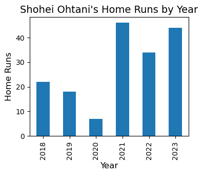
ohtani.plot(x="yearID", y="HR", kind="barh", legend=False, figsize=(4,3))

# Add chart details
plt.title("Shohei Ohtani's Home Runs by Year", fontsize=14)
plt.xlabel("Home Runs", fontsize=12)
plt.ylabel("Year", fontsize=12)


# Display the plot
plt.show()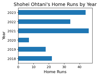
ohtani.plot(x="yearID", y=["HR", "RBI"], kind="bar", legend=False, figsize=(4,3))

# Add chart details
plt.title("Shohei Ohtani's Home Runs and RBI by Year", fontsize=14)
plt.xlabel("Year", fontsize=12)
plt.ylabel("Home Runs", fontsize=12)

# Display the plot
plt.show()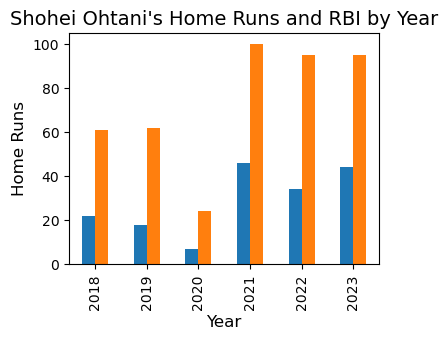
7.2 Line Graph
ohtani[["yearID", "HR", "SB"]]| yearID | HR | SB | |
|---|---|---|---|
| 75963 | 2018 | 22 | 10 |
| 75964 | 2019 | 18 | 12 |
| 75965 | 2020 | 7 | 7 |
| 75966 | 2021 | 46 | 26 |
| 75967 | 2022 | 34 | 11 |
| 75968 | 2023 | 44 | 20 |
ohtani.plot(x="yearID", y="HR", figsize=(4,3))

# Add chart details
plt.title("Shohei Ohtani's Home Runs by Year", fontsize=14)
plt.xlabel("Year", fontsize=12)
plt.ylabel("Home Runs", fontsize=12)

# Display the plot
plt.show()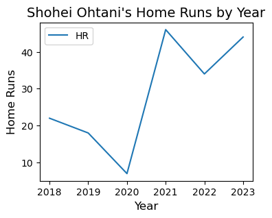
ohtani.plot(x="yearID", y=["HR", "SB"], figsize=(4,3))

# Add chart details
plt.title("Shohei Ohtani's Home Runs and Stolen Bases by Year", fontsize=14)
plt.xlabel("Year", fontsize=12)
plt.ylabel("Home Runs", fontsize=12)

# Display the plot
plt.show()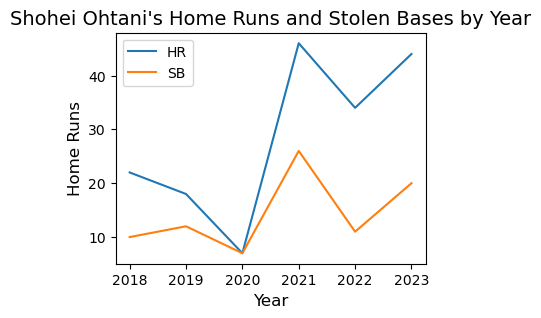
7.3 Pie Graph
ohtani.set_index('yearID')['HR']yearID
2018 22
2019 18
2020 7
2021 46
2022 34
2023 44
Name: HR, dtype: int64ohtani.set_index('yearID')['HR'].plot(kind="pie")
# Add chart details
plt.title("Shohei Ohtani's Home Runs by Year", fontsize=14)
plt.xlabel("Year", fontsize=12)
# Display the plot
plt.show()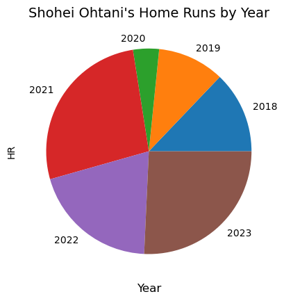
ohtani.set_index('yearID')['HR'].plot(kind="pie", autopct='%1.1f%%')

# Add chart details
plt.title("Shohei Ohtani's Home Runs by Year", fontsize=14)
plt.xlabel("Year", fontsize=12)

# Display the plot
plt.show()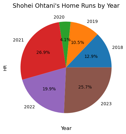
7.4 Advanced Statistics
ohtani2 = ohtani.copy()ohtani[["yearID", "AB", "H", "2B", "3B", "HR", "BB"]]
ohtani2["AVG"] = ohtani["H"] / ohtani["AB"]7.5 Histogram
angels_2023 = mlb[(mlb["yearID"] == 2023) & (mlb["teamID"] == "LAA") & (mlb["AB"] != 0)]
angels2023[["AB", "H", "HR"]]| AB | H | HR | |
|---|---|---|---|
| 506 | 39 | 5 | 0 |
| 641 | 58 | 12 | 3 |
| 14384 | 53 | 11 | 1 |
| 22036 | 50 | 10 | 1 |
| 27498 | 485 | 127 | 26 |
| 29746 | 178 | 39 | 2 |
| 32202 | 89 | 22 | 2 |
| 39328 | 194 | 42 | 8 |
| 56909 | 51 | 11 | 2 |
| 70478 | 311 | 87 | 14 |
| 72090 | 237 | 56 | 8 |
| 73970 | 289 | 65 | 9 |
| 75957 | 182 | 43 | 14 |
| 75968 | 497 | 151 | 44 |
| 76017 | 2 | 0 | 0 |
| 77621 | 8 | 1 | 0 |
| 78097 | 40 | 4 | 0 |
| 80689 | 63 | 11 | 3 |
| 84995 | 148 | 35 | 2 |
| 85004 | 459 | 111 | 19 |
| 85012 | 394 | 104 | 16 |
| 91314 | 109 | 30 | 1 |
| 96644 | 9 | 2 | 0 |
| 97961 | 62 | 18 | 0 |
| 101636 | 262 | 56 | 9 |
| 103699 | 308 | 81 | 18 |
| 104500 | 214 | 64 | 2 |
| 105414 | 81 | 14 | 2 |
| 106998 | 157 | 31 | 7 |
| 107153 | 104 | 13 | 4 |
| 107485 | 356 | 90 | 14 |
import matplotlib.pyplot as plt
from matplotlib.ticker import MaxNLocator

# Calculate the number of bins based on the data range and desired bin width
bin_width = 5
min_hr = 0
max_hr = angels_2023["HR"].max()
bins = range(0, int(max_hr) + bin_width, bin_width)

# Plot the histogram with specified bin width
angels_2023["HR"].plot(kind="hist", bins=bins)

# Add chart details
plt.title("Angels' Home Runs in 2023", fontsize=14)
plt.xlabel("Home Runs", fontsize=12)
plt.ylabel("Player Number", fontsize=12)

# Ensure y-axis has whole number ticks
plt.gca().yaxis.set_major_locator(MaxNLocator(integer=True))

# Show the grid
plt.grid(True)

# Display the plot
plt.show()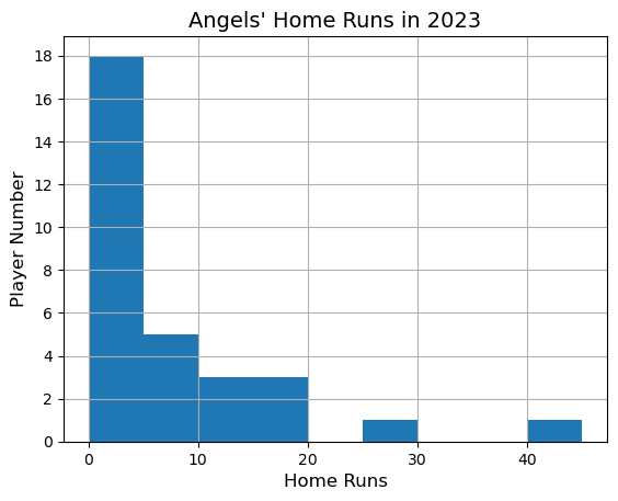
# show first few rows
mlbpost.head()| yearID | round | playerID | teamID | lgID | G | AB | R | H | 2B | ... | RBI | SB | CS | BB | SO | IBB | HBP | SH | SF | GIDP | |
|---|---|---|---|---|---|---|---|---|---|---|---|---|---|---|---|---|---|---|---|---|---|
| 0 | 1884 | WS | becanbu01 | NY4 | AA | 1 | 2 | 0 | 1 | 0 | ... | 0 | 0 | 0 | 0 | 0 | |||||
| 1 | 1884 | WS | bradyst01 | NY4 | AA | 3 | 10 | 1 | 0 | 0 | ... | 0 | 0 | 0 | 1 | 0 | |||||
| 2 | 1884 | WS | carrocl01 | PRO | NL | 3 | 10 | 2 | 1 | 0 | ... | 1 | 0 | 1 | 1 | 0 | |||||
| 3 | 1884 | WS | dennyje01 | PRO | NL | 3 | 9 | 3 | 4 | 0 | ... | 2 | 0 | 0 | 3 | 0 | |||||
| 4 | 1884 | WS | esterdu01 | NY4 | AA | 3 | 10 | 0 | 3 | 1 | ... | 0 | 1 | 0 | 3 | 0 |
5 rows × 22 columns
mlbpost.columnsIndex(['yearID', 'round', 'playerID', 'teamID', 'lgID', 'G', 'AB', 'R', 'H',
'2B', '3B', 'HR', 'RBI', 'SB', 'CS', 'BB', 'SO', 'IBB', 'HBP', 'SH',
'SF', 'GIDP'],
dtype='object')